This post is inspired by a question that one of the blog reader asked me recently. The question was related to Ms-Excel. Here is the question
I have 3 spreadsheets, Sheet1 and Sheet2. I need to copy the info from A18 in Sheet1 to A1 in Sheet2 (=Sheet1!A18) I know that is the correct formula. But I now need to copy the subsequent 7 blocks…A18, A25, A32, A39… ect for over 4000 values (meaning I can’t do it by hand). I m sure the formula looks something like this =Sheet1!A18+7… but that does not work. Any help would be greatly appreciated
I have used Ms-Excel and have done some VBA coding as well. So the very first thing that strike to me is that we can write few line of code in VBA and we can accomplish it. On a second thought, I tried to search is there a way in excel that we can achieve this.
The finding was quite interesting and it educated me with two important functions of Ms-Excel.
1. ROW()
2. INDEX()
Let us first see what the problem was and how we resolved it. For the demonstration purpose I have created an excel file with following data into it.

The user has two sheets into Ms-Excel. Sheet1 contains data that user want to copy to Sheet 2. The trick here is that user wants to start copying data from A18 cell in Sheet1. Then he/she wants to copy next 7 subsequent blocks of data i.e. A25, A32, A39, A46, A52, A59, and A66 and so on. The sheet1 has 4000 records into it.
Do you think Ms-Excel has any function or formula to copy data in this fashion? If your answer is No – (just like me before writing this post) – please read on.
Ms-Excel has two functions that are kind of magical to solve this issue.
ROW([reference]): The ROW() function returns the row number. So if you write formula "= ROW()" into A5 cell of Sheet1, this will return 5 i.e. 5th Row. The reference parameter is optional. If you pass a reference, it will always take the starting row number in the reference. For example, if we write =ROW(E10:L20), this will return 10 i.e. 10th row. Take some more example, the function =ROW(K3:S27) will return row 3 i.e. 3rd row.
INDEX(array, row_num, col_num): This INDEX() function returns specific value or the reference to a value from the range. For example, if you want to return specific value 36 from following data, you will pass parameters to INDEX function like =INDEX(A2:A6,3,1), where A2:A6 is array or range, 3 is row number and 1 is column number.

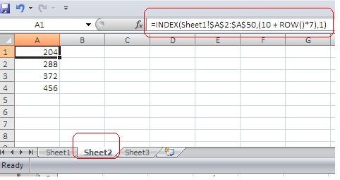
So to solve the user issue the ROW() and INDEX() together founded a solution. The solution is user can apply function =INDEX(Sheet1!$A$2:$A$50,(10 + ROW()*7),1) into Sheet2.
What we are doing with this function is we are taking data range A2 to A50 and putting
10+ ROW()*7 = 10+1*7=17th row data in first cell of Sheet2
10+ ROW()*7 = 10+2*7=24th row data in second cell of Sheet2
10+ ROW()*7 = 10+3*7=31st row data in third cell of Sheet2.
The same function can be written as =INDEX (Sheet1!$A$18:$A$50,ROW()*7-6,1)
Is not this better then writing VBA code?
PS: The solution for this question was given by Microsoft Excel Users group users actively working to solve issues like these. A big thanks goes to them. You can read the entire conversations here


