How to compare two sheets or files in Ms-Excel?

Many times we are in need to compare data of two Ms-Excel sheets. This is to find out the differences or any discrepancies in data between two sheets. In this post, I will share some of the tools and methods available to compare two sheets in Ms-Excel.

For example purpose let us consider the following excel file with data into two sheets.

Solution 1: Online Tools

www.xlcomparator.net

Xlcomparator.net is a very nice free online tool to compare two sheets. This tool supports Excel 2003, 2007 and 2010 version. You can compare two files of less than 5MB size. Once you upload the file it presents a very neat interface about what you want to compare (which columns, what is source and what is destination, ignore uppercase/lowercase etc.). This tool gives you option to download a file which contains all the mismatch or discrepancies data.

There are other online tools available to compare data between two excel files. Some of them are free and for few you have to pay but you can download the evaluation version to see if it useful for your or not. Some examples are here:

• www.speadsheetdetective.com
  
• www.synkronizer.com
  
• Beyond Compare 3

Solution 2: VBA Solution

You can use the following VBA code shared by Graham Stent to compare two sheets. For example I have a excel file with data in two sheets available. The discrepancies data are also highlighted.

I pressed the ALT + F11 to switch to VBA and pasted the below code in Sheet1. I run the UseCompareWorksheets() function and it neatly pointed out the differences in data. You can use the same to compare data in two different excel files as well

Sub UseCompareWorksheets()

'[compare two different worksheets in the active workbook]
CompareWorksheets Worksheets("Sheet1"), Worksheets("Sheet2")


'[compare two different worksheets in two different workbooks]
' CompareWorksheets ActiveWorkbook.Worksheets("Sheet1"), _
' Workbooks("WorkBookName.xls").Worksheets("Sheet2")

End Sub


Sub CompareWorksheets(ws1 As Worksheet, ws2 As Worksheet)

Dim r As Long, c As Integer
Dim lr1 As Long, lr2 As Long, lc1 As Integer, lc2 As Integer
Dim maxR As Long, maxC As Integer, cf1 As String, cf2 As String
Dim rptWB As Workbook, DiffCount As Long

Application.ScreenUpdating = False
Application.StatusBar = "Creating the report..."
Set rptWB = Workbooks.Add
Application.DisplayAlerts = False

While Worksheets.Count > 1
Worksheets(2).Delete
Wend

Application.DisplayAlerts = True

With ws1.UsedRange
    lr1 = .Rows.Count
    lc1 = .Columns.Count
End With

With ws2.UsedRange
    lr2 = .Rows.Count
    lc2 = .Columns.Count
End With

maxR = lr1
maxC = lc1

If maxR < lr2 Then maxR = lr2

If maxC < lc2 Then maxC = lc2

DiffCount = 0

For c = 1 To maxC
    Application.StatusBar = "Comparing cells " & Format(c / maxC, "0 %") & "..."
    For r = 1 To maxR
        cf1 = ""
        cf2 = ""
        On Error Resume Next
        cf1 = ws1.Cells(r, c).FormulaLocal
        cf2 = ws2.Cells(r, c).FormulaLocal
        On Error GoTo 0
        If cf1 <> cf2 Then
            DiffCount = DiffCount + 1
            Cells(r, c).Formula = "'" & cf1 & " <> " & cf2
        End If
    Next r
Next c
'**************************************
' Formating Report for Good visibility
'**************************************

Application.StatusBar = "Formatting the report..."
With Range(Cells(1, 1), Cells(maxR, maxC))
            .Interior.ColorIndex = 19
        With .Borders(xlEdgeTop)
            .LineStyle = xlContinuous
            .Weight = xlHairline
        End With
        With .Borders(xlEdgeRight)
            .LineStyle = xlContinuous
            .Weight = xlHairline
        End With
        With .Borders(xlEdgeLeft)
            .LineStyle = xlContinuous
            .Weight = xlHairline
        End With
        With .Borders(xlEdgeBottom)
            .LineStyle = xlContinuous
            .Weight = xlHairline
        End With
        On Error Resume Next
        With .Borders(xlInsideHorizontal)
            .LineStyle = xlContinuous
            .Weight = xlHairline
        End With
        With .Borders(xlInsideVertical)
            .LineStyle = xlContinuous
            .Weight = xlHairline
        End With
        
        On Error GoTo 0
End With

Columns("A:IV").ColumnWidth = 20
rptWB.Saved = True

If DiffCount = 0 Then
    rptWB.Close False
End If

Set rptWB = Nothing
Application.StatusBar = False
Application.ScreenUpdating = True
MsgBox DiffCount & " cells contain different formulas!", vbInformation, _
"Compare " & ws1.Name & " with " & ws2.Name
End Sub

Differences were shown neatly in data.

Solution 3: Excel built-in Solution

There is a very good solution provided in MSDN Forum to compare data in two excel files. The solution is to use to copy data into one excel sheet and on a third sheet use the following formula. For the best result you can sort your data before apply the formula.

=SheetName1!ColumnRowNumber= SheetName2!ColumnRowNumber

For the excel file shown above I applied the below formula and it shows True and False for the values where data has matched and not matched respectively

=Sheet1!D1=Sheet2!D1

Solution 4: Excel 2013

If you are using Ms-Office 2013, there is an in-built option to compare two sheets.

Excel 2013 > Menu Inquire > Compare files
I do not have Excel 2013 so I have not tested it

There are other solutions also which uses VLookup, HLookup, IF, Count() function. But it depends on the data and complexity that you have to go with a particular solution.

How to use Ms-Excel function SUMIFS()?

SUM and SUMIF function are very common and useful for the people who deal with Ms-Excel. Ms-Excel has a wide range of functions. Recently I learn about SUMIFS() function.

SUMIFS was introduced with MS-Excel 2007 and it works similar to SUM and SUMTIF i.e. it returns sum total of rows. The best thing about SUMIFS is it gives us functionality to apply multiple filtering criteria. It mainly has three parameters.

SUMIFS(sum_range, criteria_range1, criteria)

In the sum_range parameter we need to supply the cell range or column for which we want to return sum total.. If your entire data is in 5 rows and 5 columns (A to E column) and you want to return Sum of 5th column then you can pass E1:E5 as sum_range parameter.

In the criteria parameter we need to supply the condition or data that we are searching for. The best thing about criteria parameter is it accepts string and logical expression(>, <, =).

Let us understand it with a basic example. We have following data in the excel sheet.

Now if we have to find out sum total of Quantity Vendor Samsung supplies. We can use SUMIFS() function. We can pass the three parameters as discussed above.

=SUMIFS(E3:E18,$C$3:$C$18,"=Samsung")

This will return a sum total of 190 So Samsung is the vendor who is supplying 190 items in quantities.

Now, let us find out the sum total of quantity that Samsung supply which costs above $200

=SUMIFS(E3:E18,$C$3:$C$18,"=Samsung",D3:D18,">200")

This will return a sum total of 156. So Samsung is the vendor for 156 items which costs more than $200.

Now, let us find out sum total of products that Samsung supply which costs above $200 and item quantity is more than 80.

=SUMIFS(E3:E18,$C$3:$C$18,"=Samsung",D3:D18,">200",E3:E18,">80")

This will return a sum total of 90. So Samsung is the vendor who is supplying 90 items of for two products which costs more than $200 and has quantity more than 10.

So as you can see SUMIFS() function can accepts multiple criteria. It supports up to 27 range and criteria.

The important thing to consider about SUMIFS function is that the range should be same in all multiple criteria that we apply.

How to use Ms-Excel function COUNTIFS()?

COUNT and COUNTIF function are very popular and useful for the people who deal with Ms-Excel. Ms-Excel has a wide range of functions. Recently I learn about COUNTIFS() function.

COUNTIFS was introduced with MS-Excel 2007 and it works similar to COUNT and COUNTIF i.e. it returns number of rows. The best thing about COUNTIFS is it gives us functionality to apply multiple filtering criteria. It mainly has two parameters.

COUNTIFS(Range, criteria)

In the range parameter we need to supply the cell range of data that we are searching for. If your entire data is in 5 rows and 5 columns then you can pass A1:E5 as range parameter. In the criteria parameter we need to supply the condition or data that we are searching for. The best thing about criteria parameter is it accepts string and logical expression(>, <, =).

Let us understand it with a basic example. We have following data in the excel sheet.

Now if we have to find out number of items Vendor Samsung supplies. We can use COUNTIFS() function. We can pass the two parameters as discussed above.

=COUNTIFS(B3:E18,"=Samsung")

This will return a row count of 3. So Samsung is the vendor for three products.

Now, let us find out how many products Samsung supply which costs above $200

=COUNTIFS($C$2:$C$18,"=Samsung",$D$2:$D$18,">200")

This will return a row count of 2. So Samsung is the vendor for two products which costs more than $200.

Now, let us find out how many products Samsung supply which costs above $200 and quantity is more than 10.

=COUNTIFS($C$2:$C$18,"=Samsung",$D$2:$D$18,">200",$E$2:$E$18,">50")

This will return a row count of 2. So Samsung is the vendor for two products which costs more than $200 and has quantity more than 10.

So as you can see COUNTIFS() function can accepts multiple criteria. It supports up to 27 range and criteria.

The important thing to consider about COUNTIFS function is the range should be same in all multiple criteria that we apply.

Ms-Excel: The ROW() and INDEX() function story

This post is inspired by a question that one of the blog reader asked me recently. The question was related to Ms-Excel. Here is the question

I have 3 spreadsheets, Sheet1 and Sheet2. I need to copy the info from A18 in Sheet1 to A1 in Sheet2 (=Sheet1!A18) I know that is the correct formula. But I now need to copy the subsequent 7 blocks…A18, A25, A32, A39… ect for over 4000 values (meaning I can’t do it by hand). I m sure the formula looks something like this =Sheet1!A18+7… but that does not work. Any help would be greatly appreciated

I have used Ms-Excel and have done some VBA coding as well. So the very first thing that strike to me is that we can write few line of code in VBA and we can accomplish it. On a second thought, I tried to search is there a way in excel that we can achieve this.

The finding was quite interesting and it educated me with two important functions of Ms-Excel.

1. ROW()
2. INDEX()

Let us first see what the problem was and how we resolved it. For the demonstration purpose I have created an excel file with following data into it.

The user has two sheets into Ms-Excel. Sheet1 contains data that user want to copy to Sheet 2. The trick here is that user wants to start copying data from A18 cell in Sheet1. Then he/she wants to copy next 7 subsequent blocks of data i.e. A25, A32, A39, A46, A52, A59, and A66 and so on. The sheet1 has 4000 records into it.

Do you think Ms-Excel has any function or formula to copy data in this fashion? If your answer is No – (just like me before writing this post) – please read on.

Ms-Excel has two functions that are kind of magical to solve this issue.

ROW([reference]): The ROW() function returns the row number. So if you write formula "= ROW()" into A5 cell of Sheet1, this will return 5 i.e. 5th Row. The reference parameter is optional. If you pass a reference, it will always take the starting row number in the reference. For example, if we write =ROW(E10:L20), this will return 10 i.e. 10th row. Take some more example, the function =ROW(K3:S27) will return row 3 i.e. 3rd row.

INDEX(array, row_num, col_num): This INDEX() function returns specific value or the reference to a value from the range. For example, if you want to return specific value 36 from following data, you will pass parameters to INDEX function like =INDEX(A2:A6,3,1), where A2:A6 is array or range, 3 is row number and 1 is column number.

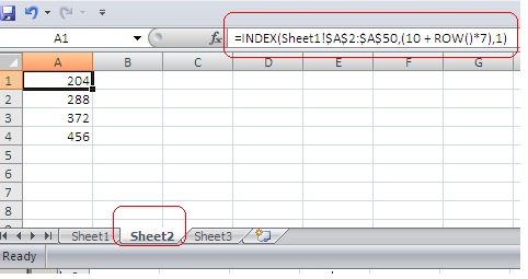
So to solve the user issue the ROW() and INDEX() together founded a solution. The solution is user can apply function =INDEX(Sheet1!$A$2:$A$50,(10 + ROW()*7),1) into Sheet2.

What we are doing with this function is we are taking data range A2 to A50 and putting

10+ ROW()*7 = 10+1*7=17th row data in first cell of Sheet2
10+ ROW()*7 = 10+2*7=24th row data in second cell of Sheet2
10+ ROW()*7 = 10+3*7=31st row data in third cell of Sheet2.

The same function can be written as =INDEX (Sheet1!$A$18:$A$50,ROW()*7-6,1)

Is not this better then writing VBA code?

PS: The solution for this question was given by Microsoft Excel Users group users actively working to solve issues like these. A big thanks goes to them. You can read the entire conversations here

Related Article:

• Ms-Excel: The ROW() and INDEX() function story
• Excel: How to use WebQuery with Excel 2007?
• Mr. vLookup() you are awesome!!!
• Ms-Excel Lookup() function …What you must know?

Mr. vLookup() you are awesome!!!

Ms-Excel world is amazing in itself. I believe we spend a lot of our life's precious time dealing with computers, laptops, I-Pad and various other gazettes. We spend a lot of time dealing with ms-office or similar products. Ms-Excel world in the form of rows and columns offers, so many functionalities that sometime we realized that there is a lot to learn about these basic software’s.

Ms-Excel in its kitty has a rich library of functions and formulas which helps in our daily routines. Recently I came to know about one of superman function of Ms-Excel “vLookup”.

vLookup() stands for Vertical Lookup. This function searches for values vertically that is in a column row after row.

What does the vLookup() function do?

vLookup() function searches for a value in a RANGE/list/column(s) and returns the corresponding value from the right side columns. That is it gives you the facility to search for a string or value in a list and you can specify what values from the right side columns you want to return. This will be clear from an example. Let us say we have data like this in our excel sheet.

Using vLookup() we can search of any employee about his Age, Dept or Salary. Our RANGE/list in this case will be all columns (Empname, age, dept and salary) and all rows. We can specify any employeeName in the search criteria of vLookup() and return any columns(age, dept or salary) from the right side . The vLookup() will search in the very first column i.e. in EmpName. For example if I have to return salary of “Vijay” the vLookup() function will take following parameter:

=VLOOKUP("Vijay",B3:E6,4)

Wild card searches with vLookup

One of the interesting fact about vLookup() function is that it gives the flexibility to search with wild card character. If you are not sure about the search value, you can use the wild card character(*,?) to search with. That is if you want to search in above shown data for salary of employee, starting with “S” character you can write the vLookup formula like this:

=VLOOKUP("S*",B3:E6,4,FALSE)

You can apply the “*” (represent any character) and “?” (represent one character) wild card character to search for values in Range/colum(s). So if you want to search for employee salary having only three character in his name, vLookup() will work for you as following:

=VLOOKUP("???",B2:E6,4,FALSE)

This will return the salary of “Jay”, whose name has only 3 characters.

Limitation of vLookup function.

One of the limitation of vLookup() function is that it cannot search for columns in it right side. That is it always returns the values from his left side of column.

Although, this limitation can be overlooked by placing the search column as very first column in our list or range.

Once you know and be familiar with the use of vLookup(), you will be amazed to see how this superman function when club with the other Ms-Excel function works like a charm.

Related Article:

• Ms-Excel: The ROW() and INDEX() function story
• Excel: How to use WebQuery with Excel 2007?
• Mr. vLookup() you are awesome!!!
• Ms-Excel Lookup() function …What you must know?